
How many landscaping visits does a two-crew route need to break even?
Calculate whole visits separately for each crew from paid hours, nonroute work, on-property minutes and travel. Apply seasonal availability, customer cancellations and weather loss to scheduled visits, then compare completed visits and sold person-hours with the paid roster and monthly operating break-even.
What you will produce: A crew-by-crew route ceiling, expected completed visits, sold on-property person-hours, monthly result and the full-season schedule needed for break-even.
Updated September 10, 2026 · Worked examples and editable worksheets
What to have ready
Bring the exact recurring residential maintenance scope, timed route-day records for both crews, customer addresses and service frequency, paid shifts, loading and equipment-care time, travel and access time, completed and deferred visits, weather and cancellation records, earned visit prices, visit-driven costs, the paid roster, standing operating costs and the selected depreciation or maintenance boundary.
Work through the calculation and decision
What counts as a completed property-service visit?
Count one visit only after one crew completes the agreed recurring maintenance scope for one residential property and records the earned charge. A quote, signed agreement, scheduled address, customer cancellation, weather deferral, skipped service, callback or return to correct the original work is not another completed visit.
An add-on delivered during the same stop changes earned revenue, materials and time. It does not create another visit unless it is independently scoped, scheduled, completed and charged. Keep sales tax collected for government and customer deposits outside earned visit revenue until their stated treatment applies.
How does route density become a whole-stop ceiling?
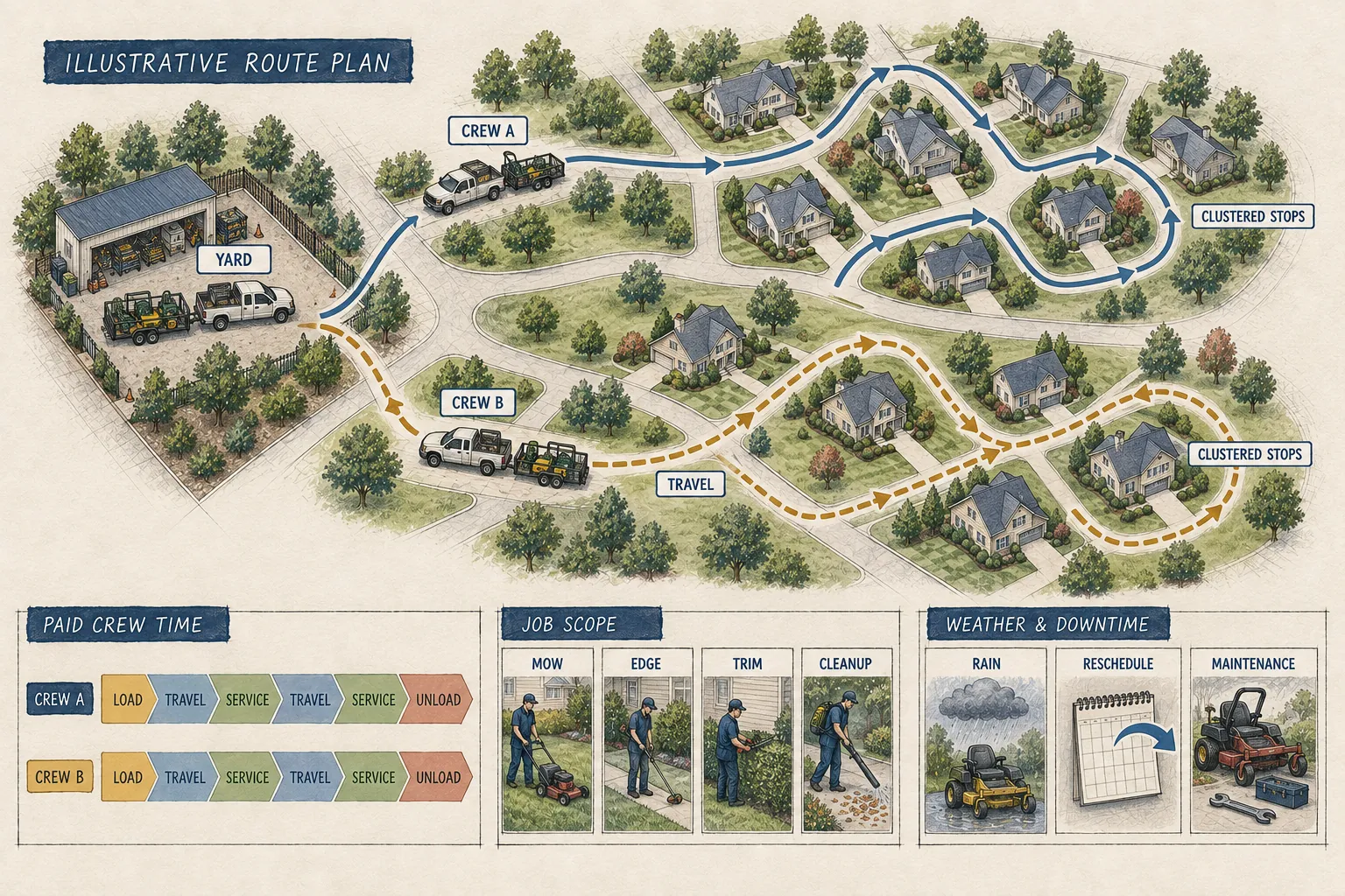
For each crew, subtract loading, breaks, equipment care, estimates and other nonroute work from the paid day. Divide the remaining minutes by on-property elapsed minutes plus travel, parking and access minutes, then round down. Calculate each crew separately because leftover minutes and equipment cannot automatically move between routes.
Translate on-property elapsed time into sold person-hours by multiplying by the workers physically assigned to that crew. A two-person crew working 45 minutes uses 1.5 person-hours. Compare sold hours with every paid field hour so travel and surrounding work remain visible.
How should seasonality, cancellations and weather change break-even?
Start with visits scheduled for a full active-season route day. Apply the share of that volume available in the modeled month, then apply customer loss and weather loss in sequence. Record recovered visits only when a later route has actual whole-stop capacity; a deferred address does not preserve revenue by itself.
Subtract the visit-driven cost from realized revenue to obtain contribution per completed visit. Divide the monthly paid-roster, occupancy, standing-cost and depreciation boundary by that contribution. Compare the resulting completed and scheduled break-even visits with both crews, and retain a separate cash plan for weak months, equipment payments, collections and tax.
The authored route completes about 307 visits and clears the entered monthly threshold by about $3,194
This teaching example uses two paid two-person crews, eight-hour route days, 90% route availability, 45 on-property minutes, nine travel and access minutes, 15 scheduled visits, 3% customer loss, 4% weather loss, 22 route days, a $105 realized price, $12.60 visit-driven cost and $25,200 fixed-cost boundary. None of these values is a national average or observed local route.
| Input or result | Calculation | Reference |
|---|---|---|
| Route minutes available per crew | 8 hours × 60 × 90% | 432 minutes |
| Whole-stop ceiling per crew | 432 ÷ (45 service + 9 travel), rounded down | 8 visits |
| Whole-company ceiling | 8 visits × 2 crews | 16 visits per route day |
| Expected completed visits per day | 15 × 97% × 96% | 13.968 visits |
| Expected monthly completions | 13.968 × 22 | 307.296 visits |
| Sold on-property person-hours | 307.296 × 45 ÷ 60 × 2 workers | 460.944 person-hours |
| Contribution per completed visit | $105.00 − $12.60 | $92.40 |
| Monthly result | 307.296 × $92.40 − $25,200 | $3,194.15 |
| Completed visits for break-even | $25,200 ÷ $92.40 | 272.73 visits per month |
| Full-season schedule needed for break-even | 272.73 ÷ 22 ÷ 97% ÷ 96% | 13.31 scheduled visits per day |
What this changes: The entered case fits its whole-stop ceiling and clears the selected threshold, but the margin depends on an unusually precise route and full seasonal availability. At 75% seasonal service volume, the same price and cost boundary produces about 230.47 completions and a $3,904.39 monthly shortfall.
Illustrative amounts are rounded for display. Use the full inputs and stated units when recalculating; an approximate threshold is not itself a sufficient activity prescription.
Keep the seasonal sensitivity attached to the same route
| Available share of full-season visit volume | Expected completed visits per month | Monthly result at the entered costs |
|---|---|---|
| 100% | 307.30 | $3,194.15 |
| 90% | 276.57 | $354.74 |
| 75% | 230.47 | −$3,904.39 |
| 50% | 153.65 | −$11,002.92 |
The table changes only seasonal service availability. It holds scheduled active-season volume, completion losses, price, variable cost and the fixed monthly boundary constant, so it is a sensitivity rather than a forecast.
Test two-crew route density, seasonal completions and break-even
Start with the worked inputs, then change a value to test your own scenario. All money amounts are in USD. The result updates in this tab.
Change travel time, seasonal volume and weather separately. Each crew keeps its own whole-stop ceiling; unused minutes in one route cannot complete a stop in another.
Calculations keep the full entered precision; displayed amounts are rounded independently. A blank, out-of-range or disallowed fractional count clears the result. Reset example restores the exact worked inputs. JSON and CSV downloads contain that same valid scenario; the worksheet download also includes your evidence and decision.
Illustrative result · assumptions apply
- Route minutes available per crew per day
- 432 minutes
- Entered service-plus-travel cycle
- 54 minutes/visit
- Travel share of the entered route cycle
- 16.67%
- Conservative whole visits per crew per day
- 8 visits/crew-day
- Conservative whole-company route ceiling
- 16 visits/day
- Expected completed visits after seasonality, cancellations and weather
- 13.97 visits/day
- Expected completed visits in the modeled month
- 307.3 visits/month
- Paid field person-hours in the modeled month
- 704 person-hours
- Sold on-property person-hours in the modeled month
- 460.94 person-hours
- Sold on-property hours as a share of paid field hours
- 65.47%
- Monthly revenue from expected completed visits
- $32,266.08
- Monthly result after entered fixed and visit-driven costs
- $3,194.15
- Approximate completed visits for monthly operating break-even
- 272.73 visits/month
- Approximate completed visits per route day for break-even
- 12.4 visits/day
- Approximate full-season scheduled visits per day required after entered losses
- 13.31 scheduled visits/day
- Whole completed visits for monthly operating break-even
- 273 visits/month
The expected completed visits cover the entered monthly cost boundary, subject to the assumptions. Whole-stop capacity is calculated separately for each crew, so leftover minutes are not transferred between routes. This exercise does not establish local demand, route time, lawful operating scope or recoverability of deferred visits.
Complete your decision record
A crew-by-crew route ceiling, expected completed visits, sold on-property person-hours, monthly result and the full-season schedule needed for break-even. Enter the finding or number, the source and the next action for each row. “Supported” records your assessment of that item; it does not approve the business or certify completed research.
| Item and what to record | Your finding and evidence | Status and next action |
|---|---|---|
| Completed-visit boundaryIncluded maintenance, property boundary, add-ons, callbacks, earned charge and collection event | ||
| Crew route-day evidenceCrew members, paid shift, loading, nonroute work, sequence, travel, access and whole completed stops | ||
| Sold person-hoursOn-property elapsed time multiplied by people assigned, kept separate from travel and all paid hours | ||
| Seasonal and completion evidenceFull-season schedule, available seasonal volume, customer cancellations, weather loss, deferred, recovered and credited visits | ||
| Price and cost boundaryRealized visit revenue, visit-driven costs, paid roster, standing costs and depreciation or maintenance counted once | ||
| DecisionBinding crew route, completed and scheduled break-even, downside case and next commitment |
6 items have no evidence recorded yet.
Entries are temporary and are not sent to us or saved automatically. Download your completed work before leaving or refreshing this page.
Choose your next action
| If your finding is… | Your next action |
|---|---|
| Break-even scheduled visits exceed either crew route or rely on transferred leftover minutes | Redesign geography, scope, cadence, price or paid cost structure and retest complete route days. |
| The result assumes deferred visits are recovered without an open whole stop | Record a credit or lost completion, add evidenced recovery capacity, or change the service agreement and cash plan. |
| A higher-priced property uses materially more service time | Compare contribution per sold person-hour and route-cycle load before expanding that property cohort. |
Errors that can change the result
- Counting scheduled, deferred or callback work as completed visits.
- Using straight-line total crew minutes when one route has unusable leftover time.
- Applying seasonality to revenue while leaving the required recovery work out of capacity.
Apply this to your business
These operating formats match the decisions in this guide.
Landscaping Company
Two two-person crews providing recurring residential landscape maintenance on compact local routes
Open the operating guide and state profiles →Carry the same visit definition, route times, paid roster, seasonal losses and cost boundary into the opening cash scenario and state reference pages. Values entered here are not automatically transferred to another calculator.
Continue with the next part of your plan
- How to plan landscaping crew capacity across routes, weather and seasons
A two-crew weekly route board, capacity and disruption ledger, seasonal staffing decision and an escalation rule for visits that cannot be recovered.
- How to price a recurring cleaning contract from its actual scope
A monthly contract-price calculation and a scope record that explains what the customer is buying.
- How to build a staffing roster before estimating payroll
A roster with complete task coverage and an annualized monthly staffing budget.
- How to build a 13-week cash plan for your first 90 days
A weekly cash schedule, the lowest balance and the extra funding needed to retain your chosen minimum.
Sources and limits
The sources below provide the stated background. The worked examples, calculator defaults and decision exercises are authored teaching material. They do not establish market prices, local demand, legal applicability or completed state research.
- U.S. Census Bureau: NAICS 561730 Landscaping Services
Official industry definition. It includes landscape care and maintenance as well as installation and design activities, so it is broader than the recurring residential maintenance format in this guide.
- U.S. Bureau of Labor Statistics: Grounds Maintenance Workers
Occupational background for landscaping and groundskeeping work. It does not establish a local hiring quote, crew productivity, lawful scope, employer cost or staffing requirement.
- U.S. Census Bureau: 2023 County Business Patterns
Employer-establishment context for NAICS 561730; it does not measure recurring residential routes, completed visits, prices, startup cost, profitability or local demand.
- IRS: state government websites
Starting links to state offices.
Source background and its scope are stated above. The guide update date does not change a source observation period. Research and review standards · Report an issue
When you need a longer financial plan
Use a financial model to organize a broader forecast after defining your own operating assumptions. The site’s research, your worksheet entries and any purchased workbook are separate; entries are not transferred automatically.